02 Jan

Lossless Audio Compression

Introduction

Here’s an audio compression scheme I came up for my tracker project. Generally, I wanted an algorithm that meets these three conditions:

  • Has to compress mono audio losslessly
  • Has to be simple, should be just one source code file or 500 lines of C code at most
  • Should compress 8-bit audio that’s upscaled to 16-bits to near 8 bits per sample

  1. Introduction
  2. The algorithm
  3. Delta encoding
  4. Gray encoding
  5. Reordering data in bit planes
  6. Run-length encoding
  7. Improvements
  8. Compression results
  9. Source code

The lossless requirement is obvious and the simplicity gives the benefit of not having to rely on external libraries (e.g. when using something like RAR compression) and not being overkill. The audio data is not huge in any case so the compression ratio doesn’t have to be exceptional. The last requirement is the most important: in klystrack, it is possible to load raw 8-bit audio files, usually originally from the Amiga computer. The native audio format in klystrack is 16-bit, however, so when saving the audio data there always are 8 redundant bits and the file will generally be twice as large as the original file. Also, since the software deals with low-fidelity aesthetics (chiptunes), the audio data might be even lower quality than 8-bit.

While there’s the option of detecting the bit fidelity and only saving the most significant bits, I thought it should be quite simple to devise an algorithm that automatically detects and leaves the redundant bits out while still doing some compression for even 16-bit audio data.

The algorithm

In short, the algorithm does this:

  1. Delta code input data

  2. Gray code the data from above

  3. Reorder the data from above in bit planes. I.e. first output the least significant bit of all samples, then the next bit for all samples and so forth

  4. Run-length encode the above data exploiting the fact you only need to store the distance between bit flips

Delta encoding

By delta encoding the audio data, we can exploit the fact audio data very often changes just a little between samples and so the generated delta values (the amount of change) need fewer bits to be expressed. However, you can’t store 16-bit data with e.g. 8-bit delta values since it is not assured the change is always small enough to be stored in 8 bits, requiring the use of 16-bit delta values in the worst case.

Gray encoding

Using gray codes we can minimize the amount of bit flipping that happens (e.g. when a value changes between 7 and 8, where the bits change from 0111 to 1000 — three bits flip even if the value changes by one) to one bit flip between any two neighboring values. In practice, this doesn’t always result in better compression and sometimes it even can hurt the compression ratio.

Reordering data in bit planes

This step is the key to good compression in our case. Between two neighboring delta values, it’s common that most of the bits are the same and it’s common for one bit to stay completely static for the whole data. So, we take the bits from all samples and sort them so that all significant bits come before the lesser bits. The result is long runs of bits, usually in the most significant bits.

Run-length encoding

Finally, we take the encoded and reordered data and store the bits using RLE. While RLE usually stores the repeated data and the number of repetitions, we can exploit the fact the data is always zero or one, always changing between runs — only the starting state of the bit needs to be stored. Elias gamma coding is used to store the run-lengths since in most cases the run length is in the range of a few bits (for completely empty bit planes we can use special flags that tell they’re all zero or one) and tend to fall in 1-4 bits. With gamma coding it’s possible to store the number 1 by using one bit, the number two takes three bits.

Also, for some bit planes a raw dump of bits with no compression should be used if compression would result in much longer data than the original. There are also two special codes for the bit planes, in cases where all bits are zero or one (common if the audio data is quiet, i.e. uses only a subrange of the 16-bit resolution) or if the data is offset by a constant.

Depending on implementation the total overhead is around two bits per bit plane (i.e. 32 bits or two bytes for 16-bit audio data), not including the header data describing the compressed data (data length, uncompressed length). Since there’s the possibility of a raw dump of bits, in the worst case (none of the bit planes compress at all), the data size grows only by two bytes. A completely quiet (all zero bits) data will take only two bytes for any length.

Improvements

My implementation only compresses the whole audio data as one big chunk but this can be easily improved to compress in chunks. This should improve the compression when there are parts where the audio is quiet and most of the bits will be zero.

Stereo audio can be compressed by compressing two chunks of data, one for both channels. The other channel should be delta coded compared to the other channel since in stereo audio the two channels often heavily correlate.

Since the Gray coding may even hurt compression, there should be the option to disable the coding for chunks. This can be simply by brute force, comparing which combination of options produces the shortest compressed data.

Compression results

The following contains example compression results. The Option column tells different configurations where the input data is delta coded and/or Gray coded. This shows how different preprocessing steps work better for different kinds of input data.

Legend: 0 = no coding before compression, 1 = delta coding, 2 = Gray coding, 3 = delta and Gray coding.

Options Ratio
Sine wave (loud)
0 73.1 %
1 29.6 %
2 67.9 %
3 22.6 %
White noise (loud)
0 100.0 %
1 100.0 %
2 99.8 %
3 100.0 %
Complex wave
0 75.3 %
1 38.2 %
2 69.6 %
3 30.0 %
Options Ratio
Sine wave and noise
0 84.7 %
1 100.0 %
2 80.9 %
3 80.9 %
White noise (quiet)
0 50.0 %
1 100.0 %
2 50.0 %
3 55.9 %
Complex wave (saturated)
0 38.9 %
1 21.9 %
2 37.2 %
3 17.7 %

Source code

#include <stdio.h>
#include <stdlib.h>
#include <string.h>
#include <math.h>

typedef unsigned char Uint8;
typedef short int Sint16;
typedef unsigned short int Uint16;
typedef int Sint32;
typedef unsigned int Uint32;


/* bitpack() bit plane codes */
enum
{
	BITPACK_STATIC0,
	BITPACK_STATIC1,
	BITPACK_LITERAL,
	BITPACK_RLE
};


/* bitstream writer helpers*/
typedef struct
{
	Uint8 *buffer;
	Uint32 byte, size_byte; 	// Read/write position counters (byte component)
	Uint8 bit, size_bit;		// Read/write position counters (bit component)
} BitPtr;

#define BIT_BLOCK_SIZE 1024 // Bitstream buffer allocation increment size

void bit_init(BitPtr *p, Uint8 *buffer, Uint32 size_bytes, Uint8 size_bits)
{
	memset(p, 0, sizeof(*p));
	p->buffer = buffer;
	p->size_byte = size_bytes;
	p->size_bit = size_bits;
}


void bit_deinit(BitPtr *p)
{
	free(p->buffer);
	memset(p, 0, sizeof(*p));
}


void bit_rewind(BitPtr *p)
{
	p->bit = p->byte = 0;
}


void bit_seek(BitPtr *p, Uint32 byte, Uint8 bit)
{
	p->byte = byte;
	p->bit = bit;
}


void bit_w(BitPtr *p, int bit)
{
	if (p->bit == 0 && !(p->byte & (BIT_BLOCK_SIZE - 1)))
	{
		// If write position modulo BIT_BLOCK_SIZE is zero, allocate a larger buffer
		p->buffer = realloc(p->buffer, p->byte + BIT_BLOCK_SIZE);
	}

	if (bit)
		p->buffer[p->byte] |= 1 << p->bit;
	else
		p->buffer[p->byte] &= ~(1 << p->bit);

	++p->bit;
	
	if (p->bit == 8)
	{
		p->bit = 0;
		++p->byte;
	}
	
	p->size_byte = p->byte;
	p->size_bit = p->bit;
}


int bit_r(BitPtr *p)
{
	if (p->size_byte <= p->byte && p->size_bit <= p->bit)
		return -1;

	int bit = (p->buffer[p->byte] & (1 << p->bit)) != 0;
	
	++p->bit;
	
	if (p->bit == 8)
	{
		p->bit = 0;
		++p->byte;
	}
	
	return bit;
}


/* Write Elias gamma coded value (has to be nonzero) */
void bit_wgamma(BitPtr *p, Uint32 value)
{
	int l = log2(value);
	
	for (int a=0; a < l; a++)
		bit_w(p, 0); //put 0s to indicate how many bits will follow
		
	bit_w(p, 1);      //mark the end of the 0s
	
	for (int a=l-1; a >= 0; a--) //Write the bits as plain binary
	{
		bit_w(p, value & 1 << a);
	}
	
}


/* Read Elias gamma coded value, zero return value signals read error */
Uint32 bit_rgamma(BitPtr *p)
{
	int numberBits = 0;
	int bit;
	while (!(bit = bit_r(p)))
		numberBits++; //keep on reading until we fetch a one...
	
	if (bit < 0) return 0;
		
	Uint32 current = 0;
	for (int a=numberBits-1; a >= 0; a--) //Read numberBits bits
	{
		if ((bit = bit_r(p)))
			current |= 1 << a;
			
		if (bit < 0) return 0;
	}
	current |= 1 << numberBits; //last bit isn't encoded!
	
	return current;
}


/* Read bits bits */
Sint32 bit_rbits(BitPtr *p, Uint8 bits)
{
	Sint32 rval = 0;

	for (int i = 0 ; i < bits ; ++i)
	{
		int bit = bit_r(p);
		
		if (bit < 0) return -1;
		
		rval |= bit << i;
	}
	
	return rval;
}


/* Write bits bits of v */
void bit_wbits(BitPtr *p, Uint32 v, Uint8 bits)
{
	for (int i = 0 ; i < bits ; ++i)
	{
		bit_w(p, v & (1 << i));
	}
}


/* Gray and delta encoding helpers */
static inline Uint16 gray(Uint16 v)
{
	return v ^ (v >> 1);
}


static inline Uint16 degray(Uint16 v)
{
	v ^= (v>>8);
    v ^= (v>>4);
	v ^= (v>>2);
	v ^= (v>>1);
	return v;
}


static void delta_encode(Sint16 *buffer, const int n)
{
	Sint32 delta = 0;
	Sint32 original;
	for (int i = 0; i < n; ++i)
	{
		original = buffer[i];
		Sint32 x = original - delta;
		buffer[i] = gray(x + 32768); // Gray code can not be negative
		delta = original;
	}
}


static void delta_decode(Sint16 *buffer, const int n)
{
	Sint32 delta = 0;
	for (int i = 0; i < n; ++i)
	{
		Sint32 v = degray(buffer[i]);
		buffer[i] = (v - 32768) + delta;
		delta = buffer[i];
	}
}


/* Compress 16-bit signed data into bitstream, return compressed data size in packed_size (in bits) */
Uint8 * bitpack(const Sint16 *_buffer, const int n, Uint32 *packed_size)
{
	BitPtr bp;
	bit_init(&bp, NULL, 0, 0);
	
	Sint16 *buffer = malloc(sizeof(Sint16) * n);
	memcpy(buffer, _buffer, sizeof(Sint16) * n);
	
	delta_encode(buffer, n);
	
	for (int plane = 0 ; plane < sizeof(*buffer) * 8 ; ++plane)
	{
		const Sint16 mask = 1 << plane;
		int bit = mask & *buffer;
		
		int type = BITPACK_STATIC0 | (bit != 0);
		
		for (int i = 0 ; i < n ; ++i)
			if ((buffer[i] & mask) != bit)
			{
				// Was not all zeros or all ones, needs to compress
				type = BITPACK_RLE;
				break;
			}
			
		Uint32 p_byte = bp.byte;
		Uint32 p_bit = bp.bit;
		
again:
		
		bit_wbits(&bp, type, 2);
			
		switch (type)
		{
			case BITPACK_LITERAL:
				for (int i = 0 ; i < n ; ++i)
					bit_w(&bp, buffer[i] & mask);
				break;
			
			case BITPACK_STATIC0:			
			case BITPACK_STATIC1:
				// No data needed, bit plane is all zeros or all ones
				break;
				
			case BITPACK_RLE:
			{
				// Write starting bit state
				bit_w(&bp, bit);
				
				Uint32 ctr = 0;
				
				for (int i = 0 ; i < n ; ++i)
				{
					if (((buffer[i] & mask) == bit))
						++ctr;
						
					if ((buffer[i] & mask) != bit)
					{
						bit_wgamma(&bp, ctr);

						ctr = 1;
						
						// Flip the bit (no neighboring bits are the same state)
						bit ^= mask;
					}
				}
				
				if (ctr != 0) bit_wgamma(&bp, ctr);
				
				if ((bp.byte * 8 + bp.bit) - (p_byte * 8 + p_bit) > n + 2)
				{
					// RLE gave longer data than the original, dump data instead
					bit_seek(&bp, p_byte, p_bit);
					type = BITPACK_LITERAL;
					goto again;
				}
				
			}	
			break;
		}
		
	}
	
	free(buffer);
	
	*packed_size = bp.byte * 8 + bp.bit;
	
	return bp.buffer;
}


/* Decompress compressed bitstream into 16-bit signed data, decompress at most packed_size bits
	unpacked_size tells the function the data length (important)
 */
Sint16 * bitunpack(const Uint8 *packed_data, const Uint32 packed_size, Uint32 unpacked_size)
{
	BitPtr bp;
	bit_init(&bp, (Uint8*)packed_data, packed_size / 8, packed_size & 7);
	
	Sint16 *buffer = calloc(unpacked_size, sizeof(Sint16));
	
	for (int plane = 0 ; plane < sizeof(*buffer) * 8 ; ++plane)
	{
		const Sint16 mask = 1 << plane;
		
		Sint32 type = bit_rbits(&bp, 2);
		
		if (type < 0) goto read_error;
			
		switch (type)
		{
			case BITPACK_LITERAL:
				for (int i = 0 ; i < unpacked_size ; ++i)
				{
					int bit = bit_r(&bp);
					if (bit < 0) goto read_error;
					if (bit) buffer[i] |= mask;
				}
				break;
				
			case BITPACK_STATIC0:
				// Data bits are zero by default, no action needed
				break;
				
			case BITPACK_STATIC1:
				// Fill bit plane with set/unset bit
				for (int i = 0 ; i < unpacked_size ; ++i)
					buffer[i] |= mask;
				break;
				
			case BITPACK_RLE:
			{
				// Read the starting bit status
				int bit = bit_r(&bp);
				
				if (bit < 0) goto read_error;
				
				if (bit) bit = mask; else bit = 0;
				
				buffer[0] |= bit;
				
				for (int i = 0 ; i < unpacked_size ; )
				{
					Uint32 ctr = bit_rgamma(&bp);
					
					if (ctr == 0) goto read_error;
					
					for (; i < unpacked_size && ctr ; ++i, --ctr)
						buffer[i] |= bit;
					
					if (ctr) goto read_error;
					
					// Flip the bit (neighboring bits are always different)
					bit ^= mask;
				}
			}		
			break;
		}
	}
	
	delta_decode(buffer, unpacked_size);
	
	if (0)
	{
read_error:
		free(buffer);
		return NULL;
	}
	
	return buffer;
}


/* Generate test data, 0 is a sine wave and 1 generates noise */
void getdata(Sint16 *buffer, const int n, int t)
{
	switch (t)
	{
		case 0:
			for (int i = 0 ; i < n ; ++i)
			{
				buffer[i] = (((int)(sin((float)i / 1000 * 3.141 * 2) * 20000)));
			}
			
			break;
			
		case 1:
			for (int i = 0 ; i < n ; ++i)
				buffer[i] = (rand() * 4);
			
			break;
	}
}


int main(int argc, char **argv)
{
	const int n = 100000;

	Sint16 *b = malloc(sizeof(Sint16) * n);
	Uint32 packed_size;
	
	getdata(b, n, 0);
	
	Uint8 * data = bitpack(b, n, &packed_size);
	Sint16 * udata = bitunpack(data, packed_size, n);
	
	if (udata == NULL || memcmp(b, udata, sizeof(Sint16) * n) != 0)
	{
		printf("Upack failed\n");
	}
	else
	{
		printf("Compression ratio %.1f %%\n", (float)100 * packed_size / (n * sizeof(Sint16) * 8));
		
	}
		
	free(data);
	free(udata);
	free(b);
	
	return 0;
}
09 Nov

Plenty of Room, Part II

This is the second part of the epic (two three-part) series of articles about tiny intros, the previous part was an essay about 256-byte intros in general.

Ed. note: Since this article seems to take forever to finish, here’s the first half of it. The (hopefully) final part will detail more of the specifics.

rubba As stated earlier, tiny intros written in assembly language fascinate me. I have written a few in x86 assembly language, here’s one of them. I have tried to make the inner workings of the program as accessible — or, at least as thought-provoking — as possible even if assembly wasn’t their weapon of choice.

I’ve included the original DOS intro (you can use DOSBox to run it, it should also work on Windows XP) and a Win32 port of it, written in C while trying to keep the original structure intact. I’ll also try to explain the general idea of the effect in pseudocode where syntax can be an obstacle. The archive rubba_c.zip contains the source code, rubba_b.exe which is the compiled Win32 executable and RUBBA.COM which is the 16-bit MS-DOS executable. To compile the C program, you need the TinyPTC library (like SDL but even more bare-bones).

I won’t go into details about x86 assembly language, I suggest anyone interested first reads an introduction and learns some of the basics. However, I’ll try to make the code look interesting, explain some weird or obfuscated code and probably show some basic size optimization tricks.

The Effect

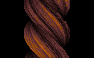
The intro, called rubba_b, shows one effect: a twisting bar drawn using primitive light-shaded texture mapping. The color palette and the texture are generated run-time. The texturing is done using linear interpolation and no vector math is used even if the bar looks like it is rotated. The lighting is an extremely simple approximation of the light source being exactly where the camera is located. That is, the length of the textured line directly determines the light.

If looked from above, the bar will be a tower of squares. If one of the squares is rotated around the center, the corners will move in a circular pattern. So, the X coordinate will be equal to cos(corner_number*(360 degrees/4)+square_rotation), the Z coordinate (why Z? Because it goes towards the screen) is equal to the sine but it can be discarded because we will not need it for perspective calculation. Remember, we’re short on bytes.

We then modulate the bar rotation for each square in the tower. If the amount of rotation changes when moving up or down the tower, the bar will twist. If the rotation stays the same for each square, the bar will rotate uniformly and look uninteresting.

The textured horizontal line is drawn from each corner to the next corner, from left to right. If the line would be drawn from right to left, we know it isn’t facing towards the camera, another line facing the camera will be drawn over it and we simply skip the line. The color value fetched from the texture is multiplied by the line length which makes short lines darker.

Still with me?

The Code

Initialization

First things first. We need to set the video mode before we continue. In the Win32 version we simply open a TinyPTC window, in the original version we need to tell BIOS to go in a nice 320x200x8 video mode (the de facto video mode back in the day).

C asm
ptc_open("rubba_b",320,200)
mov al,13h
int 10h

In the above code, the Win32 part is self-explanatory. The assembly bit probably needs some clarification: we put the number 13h (hex) in the 8-bit register al and we request for interrupt 10h. This is the BIOS video interrupt and since register ax (which consists of al – “low” – and ah – “high”) equals to 0013h (when the program starts, ax is always zeroed), BIOS will call the routine for changing the video mode (ah=00h) to 13h.

If above sounds complicated, don’t worry. It’s just a matter of memorization – similar to how you would memorize the function name for changing the video mode.

The next thing we need is some space for the texture, the sine table and the double buffer. In the Win32 version this is obvious, we just add a few arrays (although since TinyPTC only supports 32-bit video modes, we will also have an array for the palette). Again, in the assembly version we won’t use any fancy way to reserve memory to save some precious bytes: we simply decide certain areas of the memory will be used for whatever we want. The benefits of no memory protection and single tasking. ;)

C asm
short int sinetab[SINETAB];
unsigned char palette[256*4];
unsigned char texture[256*256];
unsigned char screen[320*200];
mov dh,80h
mov gs,dx           
mov dh,70h
mov es,dx
mov dh,60h
mov fs,dx

The assembly version basically sets the register dx to 60xxh-80xxh (we set only the high byte, i.e. dh to save bytes, thus the low byte of dx is undefined – it won’t matter) and puts the value into various segment registers (es-gs).

This makes it so that if we use the different segment registers, we can access each of the three 64 kilobyte segments as a 64 kilobyte array. E.g. the sine is in gs, thus mov ax,[gs:2] would move the second word in the sine table in ax. In C, the equivalent would be short int value=sinetab[1] (note how the C compiler knows the fact that a word is 2 bytes but in assembly you have to take care of that yourself – all memory accesses are always by the exact location, not the array element!).

All this is because in 16-bit memory accessing you can see only 64 kilobytes at one time. You can’t have a 128 KB array, nor can you have two 64 K arrays in the same segment. It’s something comparable to having a flashlight and a big sheet of paper in a dark room; you can move the light to show different areas but you will never see more than what there is in the spotlight.

The next two parts calculate the sine table (back in the day you simply could not do trigonometric stuff real-time, even in hardware — although in the intro it’s there just for show) and set the palette. This is pretty straight-forward stuff across the two versions. The only difference is that in the Windows version we have to remember the palette has 8-bit color components and the original has 6-bit components (0..255 ~ 0..63). And of course, the Windows version simply puts the values in a palette look-up table (because 32-bit video mode doesn’t use a palette) and the original actually sets the video mode colors.

I won’t reiterate the source code for the sine table and palette change here, I think you should be able to figure it out by comparing the source code. But in theory, here’s how to change a color: first, write the color index in port 3C8h, then write the three color components in port 3C9h (hint: dx first contains 3C8h and it’s incremented to 3C9h to save bytes).

The sine routine increases the angle (st0 the topmost register on the FPU) by 2*PI/32768 (a full circle is 2*PI, the sine table has 32768 elements). You probably should check some FPU tutorial, arithmetic on the 8087 is pretty interesting due to the stack-based architecture. For example, you first push in two numbers and then do an add, which (in most cases) pops out the two values and pushes in the result.

The texture generation bit is interesting. It also was annoying to port to C thanks to the fact you have to emulate how some instructions work – there are no accurate analogies in the C standard. A big thanks goes to baze whose code I originally cannibalized for this (I think). To be honest the conversion doesn’t work 100 % accurately but does still produce a nice texture.

The algorithm uses addition, bitwise operations and other simple things to achieve complexity thanks to how processors do arithmetics. Mainly, the results from an earlier calculation is carried over to the next calculation — when an addition or a subtraction overflows, i.e. the result is too large or too small to fit in a register, the processor lets the result wrap over but sets the carry flag.

This is quite similar to how you would carry numbers when calculating with a pen and a paper. The flag affects the results unpredictably because it’s used across quite different operations; usually you would just use to to add big numbers together as in the pen and paper example.

The Main Loop

Here is the meat of the code. The C version has many variables that are named after registers in order to see the connection with the original code. Sometimes, as with the 8-bit registers, some code doesn’t work exactly as in the original because you can’t do things similarly in C. E.g. you can’t have two variables that also are a part of one big register similarly how al and ah form ax (well, you can with pointers or unions but that is besides the point, kind of).

Self Modifying Code

I use self modifying code (SMC) in a few places because it produces faster and also much simpler code. For example, if you have a variable that is changed in a few places but used by one instruction only (and the instruction performs arithmetic or otherwise accepts a constant parameter), it’s much faster to store the variable where the constant for the instruction would be. That way you don’t have to read the variable in a register and then use the register to do something.

E.g. Let’s multiply cx by the variable foo:

Original SMC
  push ax ; save ax
  mov ax,[foo] ; move variable foo in ax
  imul cx,ax ; multiply cx by ax
  pop ax  ; restore ax
  ...
  mov ax,123   ; set foo ...
  mov [foo],ax ; ... to 123
  ...
foo: dw 0
  imul cx,123
foo equ $-2
  ...
  mov ax,123   ; set foo ...
  mov [foo],ax ; ... to 123

We can exploit the fact imul (signed multiplication) accepts constant multipliers. If you looked at the code with a hex editor, you’d see 123 next to the opcode. You can change the constant run-time and you do that exactly like you would change a variable: if you just define foo as the address where the constant is (the above code defines it as the last two bytes (i.e. word) of the previous instruction: in NASM, $ is the current location and $-2 equals the address of the previous word).

To be concluded…

02 Sep

Retargeting Images Using Parallax

I came up with a neat way to retarget images using a mesh that is transformed by rotating and doing an ortographic (non-perspective) projection. This is generally quite interesting since it can be done using a mesh and simple transformations and so can be done almost completely on the GPU. Even using a mesh can be avoided if one uses a height map à la parallax mapping to alter the texture coordinates so just one quad needs to be drawn (with a suitable fragment shader, of course).

The idea is simply to have areas of images at a slope depending of how much the areas should be resized when retargeting. The slope angle depends of from what angle the source image is viewed to get the retargeting effect since the idea is to eliminate the viewing angle using the slope.

Here’s a more detailed explanation:

  1. Create an energy map of the source image, areas of interest have high energy

  2. Traverse the energy map horizontally accumulating the energy value of the current pixel and the accumulated sum from the previous pixel

  3. Repeat the previous step vertically using the accumulated map from the previous step. The accumulated energy map now “grows” from the upper left corner to the lower right corner. You may need a lot of precision for the map

  4. Create a mesh with the x and y coordinates of each vertex encoding the coordinates of the source image (and thus also the texture coordinates) and the z coordinate encoding the accumulated energy. The idea is to have all areas of interest at a steep slope and other areas with little or no slope

  5. Draw the mesh with ortographic projection, using depth testing and textured with the source image

  6. Rotate the mesh around the Y axis to retarget image horizontally and around the X axis to retarget image vertically

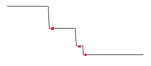
Here is a one-dimensional example (sorry for the awful images):

Source image

Source image

The red dots represent areas of interest, such as sharp edges that we don’t want to resize as much as we want to resize the areas between the details. We then elevate our line for every red dot:

red-dots

Elevated mesh

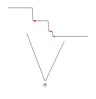
Imagine the above example as something you would do for every row and column of a two-dimensional image. Now, when the viewer views the mesh (which is drawn without perspective) he or she sees the original image:

red-dots3

Viewing the mesh from zero angle

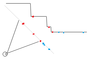
However, if the viewing angle is changed, the red dots don’t move in relation to each other as much as the areas that are not elevated when they are projected on the view plane. Consider the below example:

red-dots3

Viewing the mesh from an angle (gray line is the projected mesh)

Note how the unelevated line segments will seem shorter from the viewer’s perspective while the distance between the red dots is closer to the original distance. The blue dots in the above image show how areas that have little energy and so are not on a slope, thus will be move more compared to the red dots.

23 Jul

Collision Detection with Occlusion Queries Redux

Introduction

Here we describe a method for checking collisions between arbitrary objects drawn by the GPU. The objects are not limited to any shape, complexity or orientation. The objects that are checked for collisions can be the same objects that are drawn on the screen. The algorithm is pixel perfect but without further refining is limited to 2D collisions.

Description

The algorithm can be divided in three separate steps:

  1. Determine which objects need testing

  2. Set up the GPU buffers and draw the first object so the stencil buffer is set

  3. Make an occlusion query using the and using the stencil from the previous buffer

If the occlusion query returns any pixels were drawn, the two objects overlap.

Determining objects that need to be tested

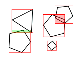
Figure 1.
Figure 1.

To speed up the algorithm, we need to eliminate object pairs that can’t overlap. This can be done by projecting the object bounding volumes in screen space. Then, we can quickly check which 2D polygons overlap and do further checking. Choosing the shape of the bounding volumes/polygons is not relevant. In this document we will use rectangles for the simplicity.

The example case in figure 1 shows two colliding objects (overlapping bounding rectangles shown red), one near hit (green overlap) and one object with no collisions or bounding rectangle overlap. To determine the collisions (and non-collisions) we need checks for every bounding rectangle (15 checks) and two checks using the GPU1. Without the use of the bounding rectangles, we would need 13 more checks on the GPU.

The bounding rectangles in the example can be generated by finding the maximum and minimum coordinates and using them as the corner points of the rectangle. Since the algorithm finds collisions as seen from the camera, we need first project the object coordinates (or the object bounding volume coordinates) on the screen and find the minima and maxima using those coordinates. Most 3D frameworks provide functions for projecting a 3D point to screen coordinates using the same transformations as seen on screen2.

Drawing objects

Before we start drawing the objects on the graphics buffer, we need to clear the stencil buffer. After that, the GPU should be set to draw only to the stencil buffer, that is we don’t need the color buffer or depth buffer to be updated.

Now, the first object can be drawn. After that, we will draw the second object. Before we start we need to set up the occlusion query to count the drawn pixels. We also need to use the stencil buffer created in the previous step and set the GPU to draw only if the stencil buffer is non-zero. We don’t need to update any buffers at this point.

After the second object is drawn, the pixel count returned by the occlusion query tells how many pixels overlap. For most purposes, we can assume a non-zero value means the two objects collide3.


Figure 2.

Figure 3.

Figure 4.

Consider the above example. Figure 2 shows two objects as seen on screen. Figure 3 shows the stencil derived by drawing only the green (right) object. Figure 4 shows what will be drawn of the red (left) object if we limit the rendering to drawing on the stencil (the occlusion query will tell us six pixels were drawn).

Sprites

For sprite objects that consist of only one quad and an alpha blended texture with transparent area representing the area that cannot collide with anything, the same result can be achieved by setting the alpha testing to discard pixels below a certain tolerance. This will then avoid updating the stencil buffer on the whole area of the quad.

Optimizations

The stencil buffer can be created to contain the collision area of e.g. every enemy currently on the screen and then testing with the player object. This avoids the necessity to test between every object individually, which can be costly since the occlusion query has to finish before the next query can start. If the objects on the screen can be grouped to a handful of categories, such as the player, the enemies, player bullets and so on, multiple objects can be tested simultaneously where it is not important to know exactly which two objects collided (e.g. when deciding whether to kill the player which in a shooter game generally is because the player collides with the background, an enemy bullet or an enemy — all of which would be drawn in the same stencil buffer).

Ideally, the above can be done so that every object group has its own stencil buffer. This then makes it possible to create the stencil and start the queries in their respective buffers, do something useful while they execute and then query for the occlusion query results.

Caveats

Most of all, doing collision detection with occlusion queries is admittedly a curiosity. There are many, many ways to do collisions faster and most likely with less technicalities. Using a simple rectangle (a cube or a sphere in 3D applications) to test collisions between complex objects has been used since the first video games and it still provides acceptable accuracy. Indeed, some games even use an extremely small collision area (e.g. a single pixel) to test collisions with larger objects with great success. Additionally, the algorithm is potentially a bottleneck, especially when triple buffering etc. are used since occlusion queries generally are started after the previous frame is drawn and then read when the next frame is drawn (i.e. it’s asyncronous). This limits either the algorithm accuracy for real time (frame accuracy) or the framerate since we may have to wait for the query to finish for a relatively long time.

A serious consideration is to use the occlusion query algorithm to test between a complex object, e.g. with a large end of level boss with a complex, changing shape and use a simpler geometry based algoritm to test between hundreds of bullets. A hybrid algorithm could even first make an occlusion query to know which objects collide and then use a different algorithm to find out more about the collision.

This is inherently a 2D algorithm. The GPU sees any situations in which two objects overlap as a collision, as seen from the location of the camera. This if fine for side-scrollers et cetera, which also benefit from pixel perfect (fair, predictable) collisions, and other situations in which all the objects to be tested are on the same plane. Multiple depth levels (e.g. foreground objects never collide with background items) improve the situation and so does drawing only the parts of the objects that are between specified depth levels4.

Another possible problem is that the screen resolution may be different between systems, which makes the algorithm have different levels of accuracy. This can be avoided by doing the checks in a fixed resolution. Limiting the collision buffer resolution also improves the algorithm speed in cases the GPU fillrate is a bottleneck.

Finally, some older systems may not support occlusion queries or stencil buffers. As of 2008, this is increasingly rare but should be taken into consideration.

Appendix A. Source code for OpenGL

The following is source code extracted from a proof of a concept/prototype game written in C++ using OpenGL. The source code should be self explanatory.

The following builds the bounding rectangle for a object:

BoundBox box=object->GetBoundingBox();

object->DoObjectTranslations();
	
glGetDoublev(GL_MODELVIEW_MATRIX, modelViewMatrix);
glGetDoublev(GL_PROJECTION_MATRIX, projectionMatrix);
glGetIntegerv(GL_VIEWPORT, viewport);

for (int i=0;i<8;i++) 
{
    GLdouble screenX, screenY, screenZ;
			
    vec3 c=box.Corner(i);

    gluProject(c.x(), c.y(), c.z(), 
        modelViewMatrix, projectionMatrix, viewport, 
        &screenX, &screenY, &screenZ);
					    
    maxX=max((int)screenX,maxY);
    maxY=max((int)screenY,maxY);
    minX=min((int)screenX,minX); 
    minY=min((int)screenY,minY);
}

rect = Rect(minX,minY,maxX-minX, maxY-minY);

The following can be used to set the rendering mode before drawing the object on the screen, on the stencil buffer or when making the occlusion query (note how we disable most of the rendering when drawing something that will not be visible to the player, also notice how the stencil buffer is cleared if we enable stencil drawing mode — using scissor makes this efficient):

void GfxManager::SetRenderMode(RenderMode mode) {
  if (mode==STENCIL) {
    glDepthFunc(GL_ALWAYS);
    glDisable(GL_LIGHTING);
    glClear(GL_STENCIL_BUFFER_BIT);	
    glEnable(GL_STENCIL_TEST);
    glDisable(GL_DEPTH_TEST);
    glStencilFunc(GL_ALWAYS, 1, 1);						
    glStencilOp(GL_REPLACE, GL_REPLACE, GL_REPLACE);				
    glColorMask(0,0,0,0);	
  } else if (mode==OCCLUSION) {
    glDepthFunc(GL_ALWAYS);
    glDisable(GL_DEPTH_TEST);	
    glDisable(GL_LIGHTING);
    glEnable(GL_SCISSOR_TEST);
    glEnable(GL_STENCIL_TEST);			
    glStencilFunc(GL_EQUAL, 1, 1);						
    glStencilOp(GL_KEEP, GL_KEEP, GL_KEEP);		
    glColorMask(0,0,0,0);			
    glBeginQueryARB(GL_SAMPLES_PASSED_ARB, m_OccId);
  } else {
    // Set normal rendering mode here (enable lighting etc.)
  }
}

Similarly, the following is used to end drawing (specifically to end the collision testing, at which the function returns the number of pixels drawn)…

int GfxManager::FinishRenderMode(RenderMode mode) {
  if (mode==OCCLUSION) {
    glEndQueryARB( GL_SAMPLES_PASSED_ARB );
    GLuint occ=0;
    glGetQueryObjectuivARB( m_OccId, GL_QUERY_RESULT_ARB, &occ);
    return (int)occ;
  } else {
    return 0;
  }
}

… using something like this:

int GfxManager::DrawObject(int oid,vec3 pos,vec3 rot,RenderMode mode) {
  SetRenderMode(mode);
  Draw3DObject(oid, pos, rot);
  return FinishRenderMode(mode);
}

This is from the main loop, it simply goes through all objects in the game. Notice how we first prepare the collision checking for the first object to be tested (i.e. create the stencil as in step 2 of the algorithm).

for (unsigned int a=0;a<m_Objects.size();a++) {
  m_Objects[a]->PrepareCollide();
  for (unsigned int b=a+1;b<m_Objects.size();b++) {
    if (m_Objects[a]->TestCollide(m_Objects[b])) {
      // We have a collision
    }	
  }
  m_Objects[a]->FinishCollide();
}

Note that DrawObject is the same method as we use to draw the visible object on the screen. The only thing that differs is that the drawing mode is set to stencil or occlusion query. Also worth noting is how we use the rectangle to set the scissor to further reduce the workload.

void GfxObject::PrepareCollide() {
  GetGfxManager()->SetScissor(this->GetBoundingRect());
  GetGfxManager()->DrawObject(m_GfxId,GetPosition(),GetRotation(),STENCIL);
}

void GfxObject::FinishCollide() {
  // We simply reset the scissor
  GetGfxManager()->SetScissor();
}

int GfxObject::DrawCollide() {
  // We could set the scissor here to even smaller area, the overlapping area
  return GetGfxManager()->DrawObject(m_GfxId,GetPosition(),GetRotation(),OCCLUSION);
}

bool GfxObject::TestCollide(Object *obj) {
  Rect a=GetBoundingRect();
  Rect b=obj->GetBoundingRect();
	
  // No need for further collision testing if the rectangles
  // don't overlap
  if (!a.TestCollide(b)) return false;
	
  // We have a collision if any pixels were drawn
  return obj->DrawCollide() > 0;
}

Links

  1. To speed up the checks done on the GPU, we can set the scissor rectangle to the overlapping area. This helps in cases in which the overlapping area is small compared to the complete area of the object.
  2. OpenGL has gluProject(), DirectX has D3DXVecProject()
  3. It may be useful to consider a larger tolerance for fairness’ sake
  4. E.g. setting the near and far clipping planes to the distance of the second object (assuming it won’t be a problem that the clipping results in objects that have a hole)
20 Feb

Let’s make a planet

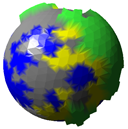
For the last few days, I have been working on a planet generator. I originally got the idea from the method how you can easily tessellate sphere into triangles. This results in a spherical map instead of a cylindrical map.

The usual way of rendering a planet as a a sphere with cylindrical texture map (or height field) looks quite bad in places because the map is stretched on the equator and pinched near the poles. The method described below takes a different approach and generates a map of vertices connected by triangles.

The vertices contain the terrain information such as terrain type (sea, land, mountain) and height. More detail is introduced by subdividing the triangles into smaller triangles.

The starting shape is an octahedron. We then subdivide each side into four triangles, normalize the new vertices and apply simple physics to move all the vertices away from the others (reverse gravity) – this eventually settles the vertices quite evenly (it won’t be a perfect shape but it is good enough for most purposes). We don’t even need to start from a symmetrical shape, using a naive repulsion algorithm eventually makes the shape symmetric as long as it is possible.

The number of subdivisions can be variable and dynamic. I’m planning to make the generator subdivide triangles on demand. In a game, you would see approximate shapes from the orbit but when flying close to the surface, the shorelines etc. would have a lot more detail. You can subdivide infinitely which means there will be infinite detail.

Dragon curve

I use a very simple algorithm to decide the terrain type on each vertex, simply the first point of the triangle decides the terrain type on the new triangle. This results into the Dragon curve fractal. A more sophisticated algorithm would change the subdivision rules according to the subdivision depth. For example, the same rules shouldn’t apply when subdividing on a continental scale versus to a scale of a few kilometers.

Next, I’m going to model a very simple simulation of atmosphere including prevailing winds, cloud formation and temperature.

Links